Decision Tree Implementation from Scratch
in Articles
In this article, we will work with decision trees to perform binary classification according to some decision boundary. We will first build and train decision trees capable of solving useful classification problems and then we will effectively train them and finally will test their performance.
The code used in this article and the complete working example can be found the git repository below:
https://github.com/fakemonk1/decision-tree-implementation-from-scratch
1. What is a Decision Tree?
Machine learning offers a number of methods for classifying data into discrete categories, such as k-means clustering.
Decision trees provide a structure for such categorization, based on a series of decisions that led to separate distinct outcomes.
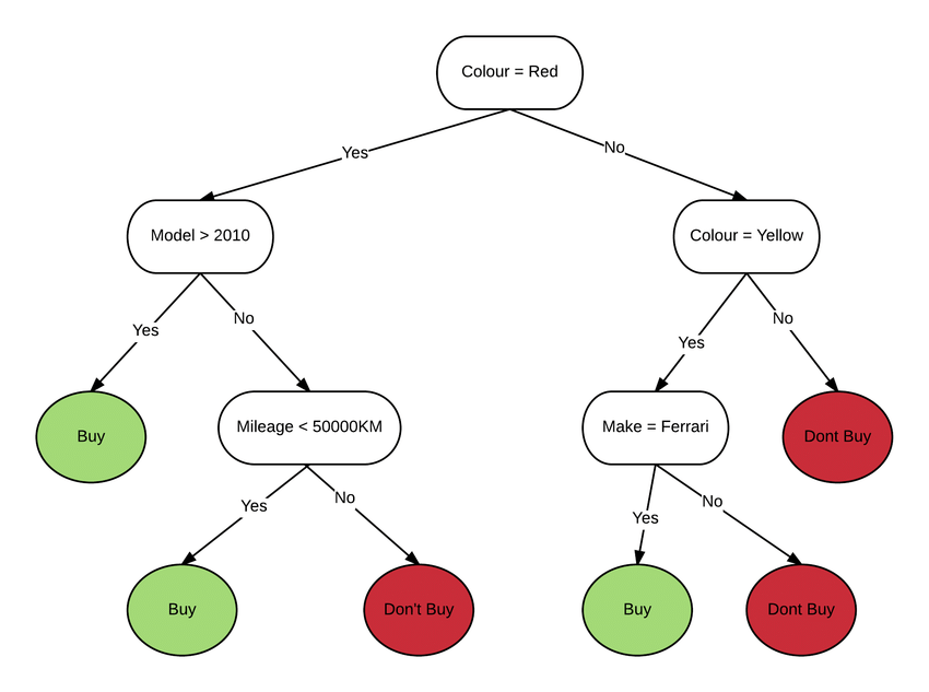
In principal DecisionTrees can be used to predict the target feature of an unknown query instance by building a model based on existing data for which the target feature values are known (supervised learning).
Following steps are taken for building the DecisionTree:
- Start with the labelled dataset containing a number of training data characterized by a number of descriptive features and a target feature
- Construct the
DecisionTreeby splitting the dataset in two recursively until the branches are pure or a stop criterion is met. - The final nodes are called leaf nodes and correspond with an output class. The rest of the nodes represent any of the input features and value of that feature which splits
the dataset - To predict the class of a new sample, the sample simply walks down the tree node by node following the split
logic until a leaf node is reached
2. How to find the best split?
In DecisionTree all the nodes are decision nodes, it means a critical decision to go to the next node is taken at these nodes.
Let us now introduce two important concepts in Decision Trees: Impurity and Information Gain. In a binary classification problem, an ideal split is a condition which can divide the data such that the branches are homogeneous. A split should be capable of decreasing the impurity in the child node with respect to the parent node and the quantitative decrease of impurity in the child node is called the Information Gain.
We need to have a unit of measure to quantify the impurity and in the information gain at each level. Common measures of impurity are Gini and Cross Entropy. Let us understand them in detail because these are prerequisite for building DecisionTree.
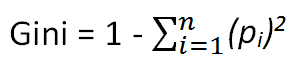
Gini Index
The Gini Index measures the inequality among values of a frequency distribution. A Gini index of zero expresses perfect equality, where all values are the same. A Gini coefficient of 1 expresses maximal inequality among values. The maximum value of Gini Index could be when all target values are equally distributed.
Steps to Calculate Gini for a split:
- Calculate Gini for sub-nodes, using formula sum of the square of probability for success and failure (p²+q²).
- Calculate Gini for split using weighted Gini score of each node of that split
Cross Entropy
For understanding Cross Entropy let us understand Entropy first. Entropy quantifies the uncertainty of chaos in the group. Higher entropy means higher the disorder. It is maximum if in a class there are an equal number of objects from different attributes (like the group has 50 red and 50 black), and this is minimum if the node is pure (like the group has only 100 red or only 100 black). We ultimately want to have minimum entropy for the tree, i.e. pure or uniform classes at the leaf nodes.
Formula of the entropy is:
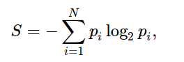
S is the current group for which we are interested in calculating entropy and Pi is the probability of finding that system in the ith state, or this turns to the proportion of a number of elements in that split group to the number of elements in the group before splitting(parent group).
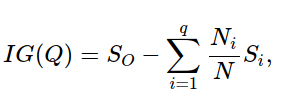
while splitting the tree we select those attributes that achieves the greatest reduction in entropy. Now, this reduction (or change) in entropy is measured by Information Gain
3. Create Split
DecisionNode is the class to represent a single node in a decision tree, which has a decide function to select between left and right nodes
class DecisionNode:

    def __init__(self, left, right, decision_function, class_label=None):
        self.left = left
        self.right = right
        self.decision_function = decision_function
        self.class_label = class_label

    def decide(self, feature):
        if self.class_label is not None:
            return self.class_label
        elif self.decision_function(feature):
            return self.left.decide(feature)
        else:
            return self.right.decide(feature)
Gini impurity is a measure of how often a randomly chosen element drawn from the class_vector would be incorrectly labelled if it was randomly labelled according to the distribution of the labels in the class_vector. It reaches its minimum at zero when all elements of class_vector belong to the same class.
def gini_impurity(class_vector):
 # Gini = 1−∑pi2
 counts = Counter(class_vector) prob_zero = counts[0] / len(class_vector) prob_one = counts[1] / len(class_vector)
 prob_sum = prob_zero ** 2 + prob_one ** 2 return 1 - prob_sum
Code to compute the gini impurity gain between the previous and current classes:
def gini_gain(previous_classes, current_classes):

    previous_gini_gain = gini_impurity(previous_classes)
    current_gini_gain = 0
    previous_len = len(previous_classes)

    if len(current_classes[0]) == 0 or len(current_classes[1]) == 0:
        return 0

    for ll in current_classes:
        current_length = len(ll)
        current_gini_gain += gini_impurity(ll) * float(current_length) / previous_len

    return previous_gini_gain - current_gini_gain
4. Build a Tree
For building the DecisionTree, Input data is split based on the lowest Gini score of all possible features. After the split at the decisionNode, two datasets are created. Again, each new dataset is split based on the lowest Gini score of all possible features. And so on, until leaf nodes are created by either max depth or min number of samples criteria.
Max depth is a parameter that controls the maximum depth until the tree can grow and is helpful in reducing the overfitting.
Every feature can be a potential split point. So we will try to split at each feature and will see spliting at which feature is resulting into lowest gini score.
 def __build_tree__(self, features, classes, depth=0):

  best_info_gain = -1
  best_column_index = -1
  best_column_threshold = -1

   if len(classes) == 0:
        return None

   elif len(classes) == 1:
        return DecisionNode(None, None, None, classes[0])

   elif np.all(classes[0] == classes[:]):
        return DecisionNode(None, None, None, classes[0])

   elif depth == self.depth_limit:
        return DecisionNode(None, None, None, get_most_occurring_feature(classes))

   else:
        for column_i in range(features.shape[1]):
            column_values_for_column_i = features[:, column_i]
            column_mean = np.mean(column_values_for_column_i)

            classes_new = []
            temp_X_left, temp_X_right, temp_y_left, temp_y_right = partition_classes(features, classes, column_i,column_mean)
            classes_new.append(temp_y_left)
            classes_new.append(temp_y_right)
            column_i_information_gain = gini_gain(classes, classes_new)

            if column_i_information_gain > best_info_gain:
                best_info_gain = column_i_information_gain
                best_column_index = column_i
                best_column_threshold = column_mean

        X_left, X_right, y_left, y_right = partition_classes(features, classes, best_column_index,best_column_threshold)
        depth += 1

        left_tree = self.__build_tree__(np.array(X_left), np.array(y_left), depth)
        right_tree = self.__build_tree__(np.array(X_right), np.array(y_right), depth)

        return DecisionNode(left_tree, right_tree,  lambda feature: feature[best_column_index] < best_column_threshold)
5. Predict the data
For predicting the target value, start with the given feature of the test dataset. Starting from the root node, evaluate the sample based on the split criteria and move to the next node. Keep traversing the tree until you are at a leaf node.
def classify(self, features):
    class_labels = []
    for feature in features:
        tree = self.root
        class_labels.append(tree.decide(feature))
    return class_labels
The code used in this article and the complete working example can be found the git repository below:
https://github.com/fakemonk1/decision-tree-implementation-from-scratch